This 1995 lecture is reviewed every year. When it is not pertinent, it will be removed. Not yet.
Planetary Boundary Layer theory remains as one of the more controversial topics in fluid mechanics. Physicists and fluid dynamacists ask fundamental questions of PBL modelers: "Why are you using the Navier-Stokes equations in turbulence regimes where they are not valid?" and "Why are you using higher order closure for turbulence when it has been proven invalid in classical fluid dynamics?" and "Why are you using K-theory diffusion equations improperly for advection in large-eddy environments?"
The Energy Transfer Group at the University of Washington answers these questions specifically in their modeling so that no inconsistency exists. This requires knowledge of basic derivations of the equations (Brown, 1991) and the nonlinear solution for the Ekman Layer (Brown, 1970, 1973, etc.). The status of this state-of-the-art of PBL modeling was discussed in the 90th AMS aniversary lecture by Brown.
Changes to our Modeling site include (10/2001; 10/2000):
The complete instability solution for the PBL perturbation equations with stratification and thermal wind and the nonlinear solution modification was completed by Foster (1996). The latent heat flux was added to the model by Brashiers (1998).
Observations from the satellite SAR (RADARSAT) show surface signatures of OLE are found about 50% of the time based on over 7000 random looks at 100km scenes of the North Pacific. The Pressure Model Function for the Satellite scatterometer indicates that the average PBL over global oceans corresponds to the nonlinear solution for the PBL with turning <U10, UG> ~ 19deg (near-neutral stratification). In general, every surface truth report of U10 or surface pressure agrees better with the nonlinear similarity solution than with numerical K-theory models.
Boundary layer and turbulence modeling: a personal perspective
R.A. Brown
Dept. of Atmospheric Sciences
University of Washington
Seattle, Washington
1. INTRODUCTION
Boundary layer and planetary boundary layer (PBL) theory are only 90 years old, 15 years older than the AMS. We have colleagues who knew the "patron Saint"; of PBL modeling, V.I. Ekman. He published his last paper, on turbulence modeling in the PBL, in 1953 (at the age of 79!). I heard a lecture by G.I. Taylor who came to Seattle in 1966. From this perspective, a lot has been accomplished in a short time. And it should be no source of shame that we still cannot do it very well (PBL modeling).
I say this up front since it seems that my role in PBL modeling is often as a critic. I don't want to appear as an overly censorous ivory-towered maven. On the other hand, I hope that I'm not dumber than the average, yet turbulence modeling often seems incomprehensible and unsatisfactory. It might help to know a little bit of my history to understand this statement. In 1962 I was a graduate student at Berkeley as TA in a boundary layer class that used higher order closure (HOC)---the 13 moment equations---to model the classic molecular boundary layer. During the course, the fact became known that the HOC equations performed worse than the Navier-Stokes equations in comparison with observations and some exact solutions. The equations apparently were not convergent and higher order approximations gave less accurate velocity profiles (than the Navier-Stokes). My professor, Sam Schaaf (Schaaf & Chambre, Flow of Rarefied Gases, Princeton Aeronautical paperbacks, 1961), declared that this was the last time it would be taught. He knew how to make political decisions, and became mayor of Berkeley. I went on to study geophysical fluid dynamics at the University of Washington.
There I met a visiting professor who was using HOC to model the turbulent PBL. I may have been the first, but certainly not the last, to ask him if this was a valid use of the equations. Prof. Wyngaard might give an answer to this question on Friday, and it will possibly be different from that of the 1960s.
Since then, my colleagues have mostly convinced me that turbulent motion is described by Newton's second law and is basically deterministic. On the other hand, I have convinced most of them that a fluid parcel isn't a Newtonian parcel, that most eddy-viscosity theory applications aren't Boussinesq eddy-viscosity, and the Navier-Stokes equations aren't used much in Atmospheric Sciences.
However I got sidetracked when Bob Fleagle gave me a satellite picture of cloud streets to explain for my thesis. It was obviously caused by an instability in the PBL. Several people, Stuart, Barcelon, Faller and Lilly had done the instability problem. But it was also obvious that very often these structures were staying around to get photographed. They did not grow exponentially. A nonlinear solution showed that they came to finite perturbation equilibrium. I wish that I had called them coherent structures, but they were 'finite perturbation secondary flows'. I wasn't very good at public relations. They are also Organized Large Eddies (OLE), or just rolls. I have written a summary every ten years since then (1970, 1980, Etling & Brown, 1993). Maybe this will qualify as a midterm report.
This gets back to the reasons that I say we still cannot do PBL modeling very well. It is necessary to go to the roots of fluid dynamics theory, as departures in methods of turbulence modeling take place immediately. Are the basic equations those of Navier & Stokes, or the Bernoulli brothers and Euler? The great dichotomy between numerical and analytic approaches must be addressed. The fundamental principles of scaling analysis and dimensional analysis must be mentioned.
2. 90 YEARS OF PBL THEORY
I will use a standard educational device for evolutionary history, a tree. Of course it is just my opinion that established the size of the branches, some that appear broken, and some that are just twigs. There are no leaves or fruit on my tree, this is just the scaffold for PBL work.
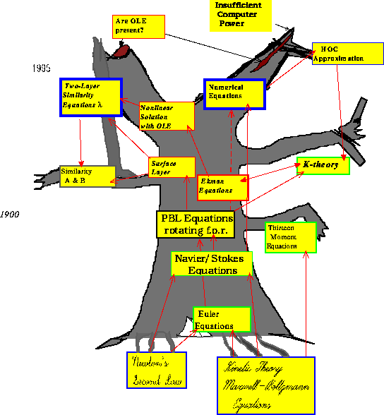
There are the kinetic theory roots of the Euler and Navier-Stokes equations. But there are also the roots in Newton's second law applied to a fluid parcel, the derivation which I have usually followed.
It all is a question of how to handle turbulence. Even of how to define turbulence. Progress has been made---for instance, the name of this meeting has been changed to Boundary Layers and Turbulence from Turbulence and Diffusion (sometimes called Turbulence and Confusion). Some scientific progress has also been made.
The questions surrounding turbulence modeling are basic. This is illustrated by the fact that debates have raged over fundamental questions: a physicists' question to Boundary Layer Meteorology, "Why are you publishing papers where the Navier-Stokes equations are being used for turbulence, where they are invalid?"; a fluid dynamist's question to higher order closure modelers, "Why are you using a procedure that failed observationally and mathematically in classical fluid mechanics"; and to the diffusion modelers, "Why are you using K-theory when it is invalid in a large-eddy environment?"; and the counter-question "So large-eddies muck up the PBL model, how often are they there?"
I have spent a lot of time on these questions. I certainly don't know the answers but I think that I can offer some partial solutions and some new challenges.
In 1905, Prandtl gave his celebrated boundary layer lecture in Heidelburg, and Ekman published his famous solution for the PBL. Prandtl's lecture introducing the boundary layer was based on scaling arguments directly. Ekman's PBL solution of 1904 had no such inspiration --- but the inherent 'thinness' of the PBL is implied from the asymptotic solution for the velocity profile. Ekman used Boussinesq's 1894 Austauch coefficient concept (eddy viscosity). His theory explained Nansen's observation that the pack ice moved at about a 45_ angle to the surface wind. His historic, elegant, and exact solution of the Navier/Stokes equations in a rotating frame of reference with three terms retained can be conveniently taught in a 50 minute lecture. This was a case in which including a rotating frame of reference provided for an analytic solution. There can be an argument over who is the 'father' of boundary layer theory. Ekman was lucky. Prandtl had better PR (H. Schlichting and his Boundary Layer Theory, 1957). Ekman still has the consolation prize of being known as one of the 'fathers of modern oceanography'.
Ninety years later both are still featured in texts, classes and papers. But there is a lot more known about the PBL. There have been some extraordinary dead-ends in theory and modeling. The 'evolutionary tree' of PBL modeling exhibits many extinctions, and has no clear 'dominant species' at present.
The simplest PBL model, and most widely used, is K, or eddy-viscosity theory. Ekman's solution applies to the ocean and atmosphere under an eddy viscosity assumption. It is still taught regularly in oceanography and atmospheric sciences classes.
However, there is a flaw in this solution....an Ekman logarithmic spiral is almost never observed. It was first often assumed that this was because K was not constant as in Ekman's basic theory, and a myriad of variable Ks were proposed to match a myriad of observed profiles. (In fact, Ekman included a variable K in his original paper.) Ekman was also an experimenter who went on excursions to measure the average flow of the PBL---hopefully, the spiral. He found, "However, analysis of the data also gave information about periodic or irregular variations of the motion" (from Kullenberg, 1954, Ekman Biography).
Finally, in the 60s, Ekman's solution was found to be unstable to infinitesimal perturbations at very low Reynolds' numbers, and thus couldn't be expected to be found in most geophysical conditions. In 1970, a nonlinear solution featuring an Ekman solution modified with organized large eddies (OLE) was completed. this solution has been used as an archtype for the general PBL solution with embedded large-eddies.
Prior to the 70s, detailed measurements were mainly confined to the surface layer of the atmosphere --- the lowest few hundred meters at most. A linearly increasing K-theory worked well to organize these data into the well-known log layer solutions for the surface layer. The plural is used because different solutions were required for variable stratification and surface roughness. These data provided the standard for flux parameterization --- the dimensionless bulk coefficients. They've been researched and documented for a wide variety of conditions, although not approaching the number of conditions in which they are used. They are employed in almost all applied models in geophysics. There are many difficulties with the accuracy of the flux coefficients (e.g. Blanc, 1987). These are compounded when bulk transfer is employed over oceans, where measurements are almost nonexistent. Nevertheless, from a PBL modeling standpoint, we will just go with the best empirical parameterizations found by the micrometeorologists.
Because of the low resolution of GCM models, the turbulent fluxes must be parameterized with respect to large scale parameters. This eliminates one of the best available methods from consideration: large eddy simulation. From numerous published critiques of point flux measurements, bulk models, GCM PBL models (Randall et al. 1993), and all other aspects of our geophysical PBL models, the state of this art is somewhat ineffectual. The chances of climate modeling accurately without this vital link are likewise deficient. New approaches are needed. We need to educate the climate modeling community.
For example, as some of you might expect, I believe that a singular event in understanding PBL dynamics came with the realization that large-eddies are innate inhabitants of the PBL. They are very difficult to measure or model. In the past decade or two, some progress has been made. We have found that when large-eddies are present, they're noxious critters, first to K-theories, then to higher order closure theories. But they do explain a lot of our difficulties.
For the first 20 years after the 'discovery' of rolls in the PBL (circa 1954), and 10 years after the analytic PBL solution containing organized large eddies (rolls), they were deemed curiosities, and relegated to appendices or footnotes, and persistently called turbulence, or 'turbulent structures'. The main accomplishment was that they explained cloud streets, the long rows of clouds at the top of the PBL, separated by a few kilometers. Then, around 1980, they were 'rediscovered' by the numerical modelers, renamed to a more generic term --- large-eddies, and revisionized. Now they are respectable, with similar appearances in both the analytic and the numerical branches of PBL analysis.
The semantic difficulties continue, and the distinction between rolls, large-eddies, OLE, coherent structures, random and organized eddies, turbulence structures and just plain old turbulence needs to be understood. It seems that the inclusion of large-eddies and thus advective rather than diffusive mixing, in a PBL model is very important, and the nuances of the large-eddies details are less important. Thus it doesn't matter so much where the large-eddies come from, dynamic or convective instabilities, random or organized, they have similar effects on the mean flow, mixing, fluxes and measurements. They need to be part of the GCM PBL. They are not at present.
However, even as a 'fringe' element of PBL modeling, there is a significant list of accomplishments for OLE modeling, with new ones found every year. Some are shown in table 1. There are also numerous applications of OLE in aerodynamics and classical boundary layers (e.g., Robinson, 1991).
The answer to the last of the basic questions posed above is becoming evident. Satellite remote sensing data is verifying the theoretical predictions of about 60% occurrence of rolls in the marine PBL. Now the other questions can be addressed. There are powerful arguments to the effect that: large-eddies are very common and part of the mean flow (of course); standard K-theory is inadequate (of course); standard HOC in GCMs is inadequate (Foster & Brown, 1994); and the Navier/Stokes equations are not useful in geophysics applications (but that's all right, we don't use them).
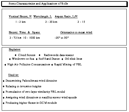
Table 1. Characteristics and Applications of OLE
Meanwhile, K-Theory practitioners have attempted to incorporate knowledge of OLE into K models. The benchmark standard for this is that of Troen and Mahrt (1986). This procedure probably encounters the same difficulties that multi-level models with much less than 50 levels invariably meet: one cannot model advection as diffusion except for very special conditions.
In the 60s, the concepts of higher order closure were being applied to the turbulent PBL. In this case, the problems of K-theory were avoided (or postponed) by replacing the Navier-Stokes equations with the nonlinear Euler equations. This approach has had two evolutionary branches. One leads to the approximations used in general circulation models, the other to the large-eddy simulations (LES). The latter can model well specific conditions, such as the cold-air outbreak done by Sykes et al. (1991). Large-eddies have been appearing in numerical models of limited domain and Reynolds' numbers since Deardorff's first models (1972). The required resolution is not likely to appear in GCMs in the foreseeable future.
In another approach, the two K-theory solutions, surface layer and Ekman, were patched together in various ways by Rossby & Montgomery (1932), Blackadar (1974, personal communication), and Brown. The one I'm most familiar with (Brown, 1974) uses a nonlinear Ekman layer solution and produces a model that uses K-theory for small eddies and explicitly parameterizes large-eddies. This analytic model extended the similarity modeling that had been constructed using dimensional analysis based on surface layer solutions, to one that included the Ekman layer. It replaced the two parameter theory with a single parameter which seems to be remarkably constant. Unfortunately, GCM modelers had already lopped off the similarity 'branch', finding the similarity theory, with two parameters A and B, inadequate.
An off-line comparison of the single parameter similarity model and a state-of-the-art HOC approximation in the Goddard Laboratories for Atmospheric Research GCM (Helfand, et al. 1991, Mellor & Yamada, 1974) suggests that the simplicity of analytic models might still be worth considering. The response of surface winds and fluxes to layer stratification was significantly different when OLE effects were included in the similarity model. Without OLE they were nearly the same. The major differences are summarized in table 2.

Table 2. Comparison between two PBL models in a GCM
Finally, if computer power increases to where Reynolds' numbers approaching geophysical values are obtainable, we can go back to the trunk, where numerical finite differencing begins, and computational fluid dynamics (e.g., Coleman et al., 1990) can be applied to the geophysical boundary layer. But until computers can handle meters resolution vertically and horizontally, Reynolds numbers around 10exp7, and can fly, I don't believe we should abandon the other main branch: analytic modeling (supplemented with numerical calculations, rather than vice versa). Currently, most of the fertilizer (funding) is flowing into the numerical branch. And possibly out of it. So there is still the struggle between the 'pure' numerical and the analytic branches.
There is a charge from climate modeling imperatives to provide an accurate parameterization of the fluxes through the PBL. It is fair to say: To reach the goals of long-term numerical weather forecasts and climate analyses, one must be able to effectively model the turbulent exchanges between the surface and the atmosphere.
Another imperative comes from the remote sensing group. First, satellite signal attenuation from temperature and humidity discontinuities associated with turbulence and coherent structures in the PBL is important. It must be calculated and accounted for in the algorithms that relate backscatter, brightness temperature or doppler lidar to geophysics parameters. Second, the geophysical applications of the microwave signal of the oceanic surface need to be be integrated --- through a PBL --- into the large-scale flow of the atmosphere at which the numerical climate models excel. Currently, backscatter signal is simply correlated to surface winds, with great success. But these winds, partly for reasons discussed here, are not a great influence on the model freestream general circulation. The PBL model is not doing the job well enough.
Before the 100th anniversary of PBL modeling, a lot of progress is going to have to be made in order to answer the questions and needs of the climate modeling and remote sensing projects. There is a real need in the PBL modeling community to make the problem known to the climate modelers.
Acknowledgments: This research was supported by NASA NAGW-2633, 2407 and 1770 and NSF ATM 8819648.
References:
Blanc, R.V., 1987: Accuracy of Bulk-method-determined Flux, Stability, and Sea Surface Roughness, J. Geophys. Res. 92, C4, 3867-3876.
Brown, R.A., 1970; A secondary flow model for the planetary boundary layer. J. Atmos. Sci., 27, 742-757.
Brown, R.A., 1974; Matching Classical Boundary Layer Solutions Toward A Geostrophic Drag Coefficient Relation. Bound.- Layer Meteor., 7, 489-500.
Brown, R.A., 1980; Longitudinal Instabilities and Secondary Flow in the Planetary Boundary Layer: A Review; Rev. of Geophysics and Space Physics, 18 (3), 683-697.
Coleman, G.N., J.H. Ferzinger and P.R. Spalart, 1990; A numerical study of the turbulent Ekman layer, J. Fluid Mech. 213, 313-348.
Deardorff, J. W., 1972, Parameterization of the PBL for use in general Circulation Models. Mon. Wea. Rev., 100, 93-106.
Ekman, V.W., 1905; On the influence of the earth's rotation on ocean currents, Arkiv. Math. Astro. Fysik., 2, 11, 1-53.
Etling, D. and R.A. Brown, 1993; A Review of Large-Eddy dynamics in the Planetary Boundary Layer, Bound.-Layer Meteor., 65, 215-248.
Foster, RC, and RA Brown, 1994: On Large-scale PBL Modeling for GCMs, A comparison between a two-layer similarity and higher order closure model, J. Global Atmos.-Ocean System, 2, 199-219, 1994.
Helfand, H.M., M. Fox-Rabinowitz, L. Takacs and A. Molod, 1991; Simulation of the planetary boundary layer and turbulence in the GLA GCM, Ninth Conference on Numerical Weather Prediction, Denver CO, October, 1991.
Mellor, G.L. and T. Yamada, 1974; A Hierarchy of Turbulence Closure Models for Planetary Boundary Layer, J. Atmos. Sci. 31, 1791-1806.
Randall, D.A., R.D. Cess, J.P. Blanchet, G.J. Boer, D.A. Dazlich, A.D. Del Genio, M Deque, V Dymnikov, V. Galin, S.J. Ghan, A.A. Lacis, H.Le Treut, Z.-X. Li, X.-Z Liang, B.J. McAvaney, V.P. Meleshdo, J.F.B. Mitchess, J.-J. Morcrette, G.L. Potter, L. Rikus, E. Roeckner, J.F. Royer, U. Schlese, D.A. Shenin, J.Slingo, A.P. Sokolov, K.E. Taylor, W.M. Washington, R.T. Wetherald, I. Yagal, and M.-H. Zhang, 1992; Intercomparison and Interpretation of surface energy fluxes in atmospheric general circulation models, J. Geophys. Res., 97, D4, 3711-3724, 1992.
Robinson, S.K., 1991; Coherent motions in the turbulent boundary layer, Annual Rev. of Fluid Mech., 23, 601-640.
Sykes, R.I., W.S. Lewellen and D.S.Henn, 1990; "Numerical simulation of the boundary layer eddy structure during the cold-air outbreak of GALE IOP-2", Mon. Wea. Rev. 118, 363-374.
Troen and L. Mahrt, 1986: A simple boundary-layer model and its sensitivity to surface evaporation., Bound.- Layer Meteor., 37, 107-128.